Abstract
It is easy to see how today’s media-rich internet runs on the JPEG algorithm just by seeing how many image file names end in “.jpeg”. Since JPEG is decades old, the fact that our internet still uses it should be strange. However, this testifies to how monumental the JPEG algorithm has been, and it deserves to be analyzed for the insights that have proved timeless. However, the algorithm itself uses dense, mathematical machinery that can be frustrating to understand. Therefore, this article tries to distill then summarize those insights, including “run-length encoding,” “Huffman coding,” and the “Discrete Cosine Transform” plus “quantization.” At the same time, it demonstrates how they work when possible. Looking at them in history, the article finally attempts to find an iterative nature to engineering.
Introduction
Arguably, today’s media-rich internet runs on JPEG. Any image online usually comes as one, and “JPEG” (along with “GIF”) has become internet lingo. That is strange, though, because it was invented in 1992 [1]—three decades ago. Many technologies from 1992 are no longer around today, so why is JPEG still used? “JPEG” refers to both a file format and an image compression algorithm, a method to make images take less space. So more fundamentally, today’s media-rich internet runs on image compression. It’s a critical technology in a world with limited computer storage and internet speeds, which is not surprising.
Rather, technologically superior formats like HEIC [2] and JPEG 2000 [3] exist, and the strange thing is that the world still runs on old JPEG. So, what led to this consensus? Perhaps it was the sheer ingenuity behind it, leading to timeless, good-enough results. Unfortunately, that ingenuity is tough to appreciate when the JPEG algorithm uses dense, mathematical machinery. Despite that, allow this article to try to show creative problem-solving using an exercise of appreciating the nature of engineering.
Level 0: Raster images
We all know that digital images aren’t like photographic film. They’re ones and zeros that can be copied, sent, and shared through computers and phones. But what is the structure of that binary data? Most digital images are “raster” images, meaning they are a two-dimensional grid of “pixels” [4]. That nature becomes obvious when zooming too far into one, finding it looks too blocky. From there, many ways exist to represent that grid as binary data—a process called encoding. That encoding is the structure.
In this article, the examples will be 16×16 grayscale images. For ease of explanation, our encoding method of choice is as follows: we will read pixels on the grid in left-to-right then top-to-bottom order, like in Figure 1. For each pixel we encounter, we will measure its brightness with a number between 0 and 255. By convention, that can be represented by eight bits, or a byte. Part of the JPEG algorithm operates directly on bits, so knowing the encoding that produced those bits helps understanding.
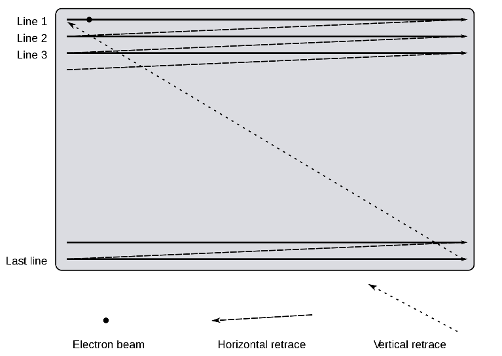
Figure 1. Raster scan pattern of a CRT screen
[https://commons.wikimedia.org/wiki/File:Raster-scan.svg]
However, if we are to cut through that machinery, we need a more tangible way to print these bits. Our approach will be to depict them as hexadecimal, with highlighting and coloring as needed. Four bits—which has 16 possible combinations: 0000, 0001, 0010, 0011, and so on—can be printed in a short-hand way called hexadecimal [5]. Instead of writing these long binary combinations, we can represent the first ten with the single-digit numbers 0 to 9. After that, to the last six combinations we assign the letters A to F. With this scheme, one pixel—encoded as eight bits—can be printed as two hexadecimal “digits”. For example, the number 120 is conventionally represented by the bits 01111000, and it can be printed instead as 78.
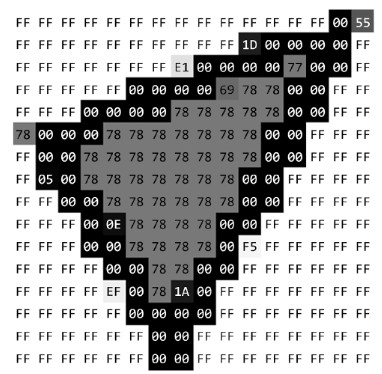
Figure 2. A series of bytes. Each byte is highlighted by the color it represents,
forming a 16×16 raster image. Graphic original.
Hexadecimal aside, our encoding scheme would mean a 12-megapixel photo would take 12 megabytes. However, JPEG applies two kinds of methods toward breaking this one-to-one rule. From information theory, “lossless” techniques seek to eliminate redundant bits—finding smaller ways to store the exact same thing. Using signal processing and psychology, “lossy” techniques seek to eliminate parts of the image in ways that would be hard to see—finding smaller ways to store something close to the same.
Level 1: Run-length Encoding
The first technique, run-length encoding, handles the low-hanging fruit. It’s not effective on all images, but on others it’s essential. At one byte per pixel, a half-grey, half-white 16×16 image would be encoded as something akin to “grey, grey, …, grey, white, white, …, white.” However, a shorter way to say the same is “128 white, 128 grey.” A computer would use one byte to store the number and another byte to store the pixel being repeated [5]. It’s simple, but (given this best-case scenario) we can already turn 64 bytes into just four.
Let us use Figure 2, though, as a more realistic example that we can carry into a later section. Using left-to-right then top-to-bottom order, we first encounter the byte FF 14 times in a row. 14 is stored (again by convention) as the byte 0E, and FF immediately follows. The complete process looks like Figure 3, where the bytes that store numbers are in green. Using run-length encoding, we have already reduced the size from 256 bytes to 130 bytes!
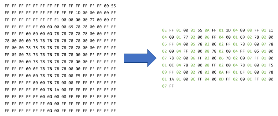
Figure 3. Demonstration of run-length encoding.
Level 2: Huffman coding
The second technique, Huffman coding, functions like Morse code. In Morse code, the most common letter (E) was represented by a single dot, the second most common (T) was represented by a single dash, then less frequent letters were represented by longer combinations of dots and dashes [6]. After a combination was tapped out, a rest period signaled that a letter had been completed. Using this approach, words were tapped out quickly.
Previously, we represented the number 120 with the bits 01111000, written as the byte 78. However, this choice was only by convention! When we look again at Figure 2, the byte 78 is visibly common, and it continues to be common in Figure 3, after run-length encoding. Like in Morse code, we should represent it with a short bit combination instead.
In this way, Huffman coding can make any data take less space by representing more common bytes with a smaller handful of bits [7]. After counting how often each byte appears, however, what bit combinations do we assign them? We know that they need to be short, but we cannot simply reuse Morse code because binary has no way to “rest”—there is no third number after one and zero. Considering this restriction, Huffman’s innovation was an algorithm that always presents the most powerful choices, mathematically guaranteed. Applying that algorithm on our running example, we get the most powerful code for reducing the run-length encoding result even further.
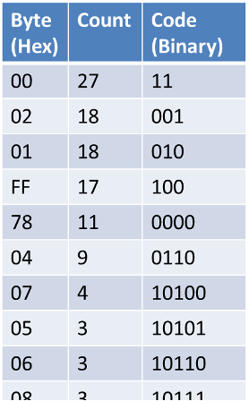
Figure 4. The code produced by Huffman coding (partial), showing more common bytes getting shorter binary combinations.
Using this code, we arrive at Figure 5, where the counts of repeated bytes are again in green.
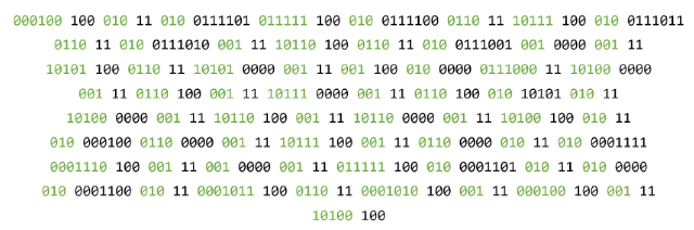
Figure 5. Result of Huffman coding on past example in binary, code absent.
We can represent this in hexadecimal again for comparison, getting Figure 6 with only a size of 59 bytes! One technicality is that the code must be included with this compressed data, but the code and compressed data together are usually smaller.
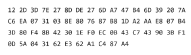
Figure 6. Result of Huffman coding on past example in hexadecimal, code absent.
Intermission: From “lossless” to “lossy” techniques
Run-length encoding and Huffman coding together are the “lossless” techniques involved in the JPEG process. These techniques alone can only effectively compress images with large, consistent regions. These would be basic digital graphics like corporate logos. Sometimes we do have that kind of image, so a variety of just “lossless” techniques get applied in PNG and GIF [8]. But sometimes we have a photograph instead, for example. Why would these techniques still be useful in the JPEG format? JPEG’s huge insight was the missing step: a “lossy” technique.
Level 3: Discrete Cosine Transform plus Quantization
That change in perspective is a transform: a mathematical method to represent data in a new way. The one used in JPEG is the Discrete Cosine Transform, or DCT. The DCT has long been a powerful tool in signal processing, and here is one of its biggest uses. The first step is splitting a photograph into many 8×8 images [1]. After that, a mathematically proven principle of the DCT is that any 8×8 image is a weighted average of some patterns called the DCT basis functions [1].
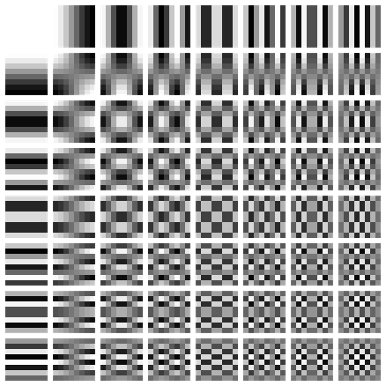
Figure 7. DCT basis functions. [https://commons.wikimedia.org/wiki/File:DCT-8×8.png]
Given a certain 8×8 image, the DCT finds these weights as an 8×8 table. In this table, the uppermost, leftmost value would correspond to the weight of the uppermost, leftmost basis function in Figure 6, and so on. Notably, the weights of the lower-right, upper-right, and lower-left “high-frequency” patterns often happen to be close to zero [1]. At the same time, this observation is helped by a psychological concept called the just-noticeable difference [9]. In short, it is the smallest difference that humans can detect, and it depends heavily on the context. In this context, studies show that our just-noticeable difference of “high-frequency” patterns is large enough that we often cannot distinguish between close-to-zero and truly zero [10]!
From here, many steps in the JPEG process are purely mathematical machinery, but it is correct to say that high frequency close-to-zero weights become truly zero [1]. This rounding effect, a part of what is called quantization, makes this technique “lossy.” At the same time, these zeroed-out weights often form a large, mostly consistent space in the 8×8 table. As a result, more mathematical machinery compresses it using the same “lossless” techniques (more or less), just as if it was an 8×8 image!
Although the “lossless” techniques were originally only useful for simple digital graphics, this technique takes any image, chops it up, then transforms the pieces into “simple digital graphics.” The result is that JPEG can usually compress any color image to a tenth of its original size [1].
Conclusion
Now, after cutting through the mathematical machinery that drives JPEG, the founding insights are easier to see. But notably, the inventors of JPEG credit run-length encoding and Huffman coding to someone else. On top of that, “lossless” image compression predated JPEG through the GIF format [8]. So, they must have simply asked: how could they extend those solutions beyond simple digital graphics? Their answer was the DCT plus quantization. It was a solution layered on a solution, yet our media-rich internet was built on this single improvement. Every file name ending in “.jpeg” testifies to that. Perhaps this could be why the new formats (like HEIC and JPEG 2000) never compelled us to replace that foundation.
But all that is hard to see when the “lossless” steps only came after using the DCT plus quantization. Without understanding, it is too easy to think of JPEG as a black box and that all the groundwork was made by the inventors alone. That is, the nature of engineering as iterative innovation can get shrouded. Instead, Rome wasn’t built in a day, and analyzing the JPEG algorithm also says Rome wasn’t built by a single person either.
References
| [1] | G. K. Wallace, “The JPEG still picture compression standard,” IEEE Transactions on Consumer Electronics, vol. 38, no. 1, pp. xviii-xxxiv, Feb. 1992. |
| [2] | “HEIC vs. JPEG,” Adobe Inc, [Online]. Available: https://www.adobe.com/creativecloud/file-types/image/comparison/heic-vs-jpeg.html. [Accessed 13 March 2022]. |
| [3] | “JPEG vs. JPEG 2000,” Adobe Inc, [Online]. Available: https://www.adobe.com/creativecloud/file-types/image/comparison/jpeg-vs-jpeg-2000.html. [Accessed 13 March 2022]. |
| [4] | “Raster Images,” University of Michigan Library, 11 February 2021. [Online]. Available: https://guides.lib.umich.edu/c.php?g=282942&p=1885352. [Accessed 13 March 2022]. |
| [5] | “Run-Length Encoding (RLE),” FileFormat, [Online]. Available: https://www.fileformat.info/mirror/egff/ch09_03.htm. [Accessed 13 March 2022]. |
| [6] | J. D. Cook, “How efficient is Morse code?,” 8 February 2017. [Online]. Available: https://www.johndcook.com/blog/2017/02/08/how-efficient-is-morse-code/. [Accessed 14 March 2022]. |
| [7] | D. A. Huffman, “A Method for the Construction of Minimum-Redundancy Codes,” Proceedings of the IRE, vol. 40, no. 9, pp. 1098-1101, Sept. 1952. |
| [8] | “LZW and Three Graphics File Formats,” Orpalis Imaging Technologies, 17 October 2019. [Online]. Available: https://www.orpalis.com/blog/lzw-three-graphics-file-formats/. [Accessed 14 March 2022]. |
| [9] | R. M. Spielman, W. J. Jenkins and M. D. Lovett, “Sensation versus Perception,” in Psychology 2e, Houston, OpenStax, 2020. |
| [10] | H. Lohscheller, “A Subjectively Adapted Image Communication System,” IEEE Transactions on Communications, vol. 32, no. 12, pp. 1316-1322, 1984. |