Abstract
Although computers have made great jumps in efficiency and speed in the past several decades, recent developments in machine learning and artificial intelligence applications are increasingly challenging the efficiency of powerful computers. The tremendous pressure in the computer hardware industry to significantly improve performance with each new generation of computer chips has traditionally followed a pattern called Moore’s Law, which states that the complexity and performance of computer chips doubles every two years. Transistors, which are small electronic components that make up computer chips, have shrunk in size with each new generation in order to keep up with Moore’s Law. However, we are now approaching a limit in which it is no longer physically possible to make transistors any smaller [23]. In other words, we are approaching a dead end when it comes to improving the performance of traditional computers. Clearly, a new approach to building computers is needed. This article proposes analog computers as a possible solution for creating new, more powerful computers in the future. It will describe how analog computers work and differ from traditional computers, as well as the benefits of analog computers in solving very complex mathematical problems.
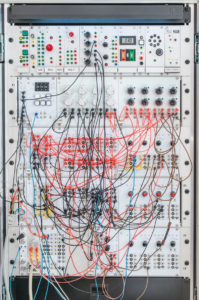
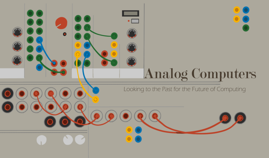
Figure 1: modern prototype of a manually configurable analog computer [12]
What is an Analog Computer?
These days, when most people think of a computer, they picture a desktop computer or a laptop. Both of these devices, along with Xboxes, smartphones, and even handheld calculators, actually belong to one specific category of computers: digital electronic computers. In reality, the definition of a computer is much broader and encompasses many other categories of devices, including analog computers.
According to Merriam-Webster Dictionary, a computer is “a programmable, usually electronic device that can store, retrieve, and process data” [1]. This definition highlights two important points about computers. First, a computer does not necessarily have to be an electronic device, even though nearly all modern computers are. Second, for a device to be considered a computer, it must be programmable and have the ability to process data.
All computers can be classified as either analog or digital. The primary difference between these two types of computers is the way in which data is represented. In a digital computer, all data is represented using a limited set of numerical values [2, p. 2]. In modern digital computers, data is represented with binary, a number system which uses only 0’s and 1’s. The simplicity of binary is both an advantage and limitation of digital computers. Long lists of binary digits are used to represent all types of data in digital computers, including text, images, and audio. However, representing data in binary form often requires approximating the data and losing some of its detail. For example, audio stored on a digital computer loses some of the quality it had when it was originally recorded [13].
Another distinct feature of digital computers is their ability to be reprogrammed to solve many different types of problems. Digital computers are configured to run an algorithm, which is essentially a list of instructions for completing a task. Another way to think of an algorithm is to consider it as a recipe for the computer to follow [24]. All digital computers run various programming languages, and these programming languages give users the flexibility to create an algorithm for any task they wish to complete.
Finally, digital computers can solve problems of virtually any level of complexity if they are given enough time to run. The more complex the problem, the longer a digital computer will take to solve it [2, pp. 3-4]. For example, imagine a digital computer is asked to sort two lists of numbers, a list with 100 numbers and a list of 1000 numbers. Due to the way a digital computer operates, it can take the computer up to 100 times longer to sort the list of 1000 numbers, even though the list is only ten times larger than the one with 100 items [20]. This inefficiency when solving certain types of problems is a major downside of digital computers, which will be further explored later in this article.
An analog computer, on the other hand, is based on an entirely different approach to solving a problem. Unlike a digital computer, the structure of the analog computer is not fixed and there is no programming language. Instead, to solve a problem, you must physically reconfigure the computer so that it forms a model, or “analog”, of the problem. When an analog computer is run, it simulates the problem and the output of this simulation provides the solution [2, pp. 3-4]. Because an analog computer is a physical model of the problem it is solving, the complexity of the problem determines the physical size of the computer. As a result, unlike digital computers, an analog computer cannot solve all problems of any complexity [2, p. 5].
To further clarify how analog and digital computers differ in the way that they solve problems, let’s consider an example in which the goal is to design a bridge and determine the maximum weight the bridge can hold. Solving this problem with a digital computer would be similar to estimating the strength of each individual beam that makes up the bridge, then analyzing how each beam interacts with the beams around it, and finally determining the total amount of weight the beams can hold together by taking into account all of their strength contributions. Using an analog computer to solve this problem is akin to building a model of the bridge and physically placing different weights on it to see which one causes the bridge to break. This example illustrates how in certain cases, using an analog computer can provide a much more direct and efficient path to the solution.
Lastly, data representation and storage differ significantly between analog and digital computers. The key difference is that in an analog computer, data can take on any value and is not restricted to being represented by a limited set of distinct values, such as binary. For example, in electronic analog computers, data is represented by electrical signals whose magnitude,or strength, fluctuates over time. The data stored in an electronic analog computer is the strength of these signals at a given instant in time. This approach allows certain types of data to be represented exactly rather than being approximated as they would in digital computers [2, pp. 31-33].
Having explored the defining characteristics of analog computers, we will now examine several examples of these computers, ranging from ancient artifacts to modern electronic systems.
Examples of Analog Computers
The first analog computers were ancient tools, one example of which is the astrolabe, which dates back to the Roman Empire. An astrolabe is a small mechanical device that was used to track the position of stars and planets. There was widespread use of this device for navigation, especially during sea travel [10].
Jumping ahead to the 20th century, we can find another example of a widely-used non-electronic analog computer: the slide rule. A slide rule was a device that assisted in performing mathematical operations between two numbers. The slide rule was marked with various scales and operations were performed by aligning the components of the device in a specific configuration. Many slide rules supported basic operations such as addition, subtraction, multiplication, and division, while others could support more complex operations such as square roots [5].
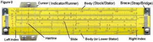
Figure 2: a slide rule with its components marked [8]
Significant advances in analog computing were made during WWII, when research and development funding ballooned due to the war effort. One example was the invention of the Turing-Welchman Bombe, a mechanical computer designed by Alan Turing to help the British crack encrypted German military messages. The Germans encrypted the messages using their own mechanical analog computer, a small, typewriter-like device called the Enigma cipher machine [2, pp. 204-211].
However, the revolution in analog computing really began with the advent of the electronic analog computer, a device in which electrical circuits–rather than physical moving parts or mechanical components–are used to model the problem being solved.
One of the pioneers of electronic analog computing was Helmut Hoelzer, a rocket scientist in Nazi Germany. Hoelzer theorized that complicated mathematical operations such as differentiation and integration could be performed more efficiently using electrical circuits. Both of these operations are from calculus and are used to calculate quantities that change over time. For example, differentiation can be used to determine how fast a rocket is accelerating by tracking its change in position over time [17].
Through his research, Hoelzer discovered that both of these operations could indeed be performed by measuring the electrical signals in a simple circuit with a capacitor. A capacitor is a basic electronic component that acts like a small battery, storing small amounts of energy and rapidly charging and discharging [16]. Hoelzer applied these revolutionary ideas to his work on the guidance system for the A4 rocket, an advanced weapon being developed by Nazi Germany which would be the world’s first ballistic missile used in warfare [9]. The guidance system that he built for the rocket was called the Mischgerät. It acquired data from the rocket’s flight sensors, performed calculations on the data using the capacitor circuits, and output a control signal which adjusted the rocket’s flight path in real-time. The Mischgerät is considered to be one of the world’s first electronic analog computers [2, pp. 34-38].
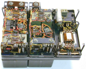
Figure 3: the Mischgerät (photo by Adri De Keijzer) [7]
As the 20th century progressed, electronic analog computers became more advanced and widely used. Institutions interested in complex mathematical simulations, such as NASA, invested heavily in them [11]. By the 1950s, there were several major companies designing and building electronic analog computers, including Electronic Associates Inc. (EAI) and Telefunken [2, pp. 101-103].
Having followed the progression of analog computers throughout history, we will now turn our focus to modern electronic analog computers and discuss their benefits and disadvantages.
Benefits and Disadvantages of (Electronic) Analog Computers
Analog computers have a variety of advantages and disadvantages in comparison to digital computers. One of the most important benefits of analog computers is that they operate in a completely “parallel” way, meaning that they can work on many different calculations at the same time.In comparison, digital computers operate sequentially and must wait for one set of calculations to complete before starting on the next set. Analog computers simulate the problem and compute the solution nearly instantaneously, while it may take a digital computer a significant amount of time to solve the same problem. To understand the difference between parallel and sequential operation, let us consider the example of trying to calculate the trajectory of a baseball given the angle and speed with which it was thrown. An analog computer will simulate all aspects of the problem simultaneously and begin outputting the trajectory of the baseball as soon as the computer is turned on. In this case, watching the output of the analog computer is like watching the baseball fly through the air in real-time. The digital computer, on the other hand, has to break the problem down into sequential steps, complete one step at a time, and then put the solutions from different steps together to come up with the final answer. After the digital computer completes its work, it will output the entire path of the baseball all at once [2, pp 249-250]. In addition to the benefits of parallel operation, analog computers do not need to access memory since they are not controlled by a stored program. Since memory accesses can significantly slow down computation, analog computers have an additional speed advantage over digital computers [2, pp 250-251].
Electronic analog computers are also particularly well-suited to solving mathematical problems which involve differentiation – specifically a group of problems called ordinary differential equations (ODEs) [2, p. 113]. ODEs are hugely important in modeling systems and phenomena in science, engineering, and a variety of other disciplines. Examples of problems that can be modeled using ODEs are population growth, the spread of epidemics, and the motion of objects – such as airplanes and rockets [3].
That said, there are several serious disadvantages to using analog computers that have hindered their adoption. First, the programming and configuration of an analog computer is specific to the structure of each individual computer. Unlike the programming languages used for digital computers, there is no convenient, standardized approach to programming analog computers. For example, while both slide rules and astrolabes are examples of analog computers, configuring an astrolabe to track the moon is quite different from configuring a slide rule to add two numbers together. Second, the size of an analog computer is determined by the complexity of the problem. For very complex problems, analog computers can become too large and intricate to build practically. Finally, data in analog computers, which is represented using electrical signals, is more susceptible to electromagnetic noise and interference. This can cause errors in the data or even corrupt the data altogether [11].
In summary, while analog computers are not as accurate or versatile as digital computers, they can greatly improve speed and efficiency for certain problem types. In the next section, we will explore recent innovations in analog computers, as well as their prospects for the future.
The Resurgence and Future of (Electronic) Analog Computers
Recent innovations in semiconductor technology are allowing us to rethink the construction of analog computers in terms of reducing their physical size and improving their computing power. Semiconductors are a group of elements on the periodic table, such as silicon and germanium,that have special electrical properties. Electronic components and circuits are usually constructed using semiconductor materials.
One revolutionary new semiconductor technology is known as very large-scale integration or VLSI. This technology enables electrical engineers to shrink down circuits to microscopic sizes. VLSI accomplishes this by fitting millions to billions of tiny electrical components on a single semiconductor chip [14]. Today, the main computer chip in a laptop, known as the central processing unit (CPU), is about the size of a cracker. Several decades ago, computers with even less computational power took up entire rooms [21].
In addition, researchers are investigating the benefits of “hybrid analog computers”, i.e. analog computers augmented with digital computing techniques that help to improve accuracy and versatility [11].
In 2015, a team of researchers at Columbia University built a “hybrid computing unit” and used VLSI technology to fit the entire hybrid analog computer onto a small computer chip. This computer is programmable and is capable of solving complex problems that can be modeled using ODEs. It is also extremely power efficient and uses only about 1.2 mW of power [4]. In comparison, a modern “low-power” CPU can use around 30 W of power. Therefore, the “hybrid computing unit” consumes around 25,000 times less power than the digital computer chip [22].
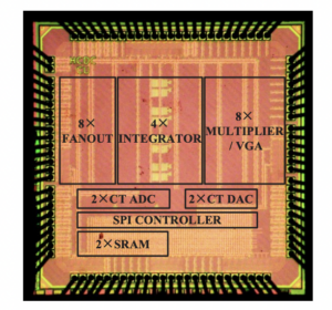
Figure 4: zoomed-in photo of the computer chip that contains the “hybrid computing unit” created by researchers at Columbia University [4]
This next generation of analog computers is particularly well-suited to meeting the pressing needs of our modern world. Science and engineering applications are demanding that we solve more and more complex mathematical problems, which can easily bog down digital computers. In addition, the power efficiency of electronics, especially in devices with limited power (such as battery powered robots), is becoming increasingly important. Analog computers are well-equipped to meet these challenges, especially as their versatility and accuracy improves with ongoing research and development.
References
[1]“Definition of COMPUTER,” Merriam-webster.com, 2019. https://www.merriam-webster.com/dictionary/computer
[2]Bernd Ulmann, Analog Computing. Walter de Gruyter, 2013.
[3]W. Trench, “1.1: Applications Leading to Differential Equations,” Mathematics LibreTexts, Jun. 07, 2018. https://math.libretexts.org/Bookshelves/Differential_Equations/Book%3A_Elementary_Differential_Equations_with_Boundary_Value_Problems_(Trench)/01%3A_Introduction/1.01%3A_Applications_Leading_to_Differential_Equations
[4]N. Guo et al., “Continuous-time hybrid computation with programmable nonlinearities,” Sep. 2015. doi: 10.1109/esscirc.2015.7313881.
[5]“Slide Rules,” National Museum of American History. https://americanhistory.si.edu/collections/object-groups/slide-rules#:~:text=Slide%20rules%20are%20analog%20computing (accessed Nov. 01, 2022).
[6]L. Gladwin, Alan Turing, Enigma, and the Breaking of German Machine Ciphers in World War II. 1997.
[7]“Archive 3 displays 5,” www.cdvandt.org. https://www.cdvandt.org/archive_3_displays_5.htm (accessed Nov. 01, 2022).
[8]D. Ross, “Illustrated Self-Guided Course On How To Use The Slide Rule,” sliderulemuseum.com, 2018. https://sliderulemuseum.com/SR_Course.htm (accessed Nov. 01, 2022).
[9]D. Day, “The V-2 (A4) Ballistic Missile Technology,” www.centennialofflight.net. https://www.centennialofflight.net/essay/Evolution_of_Technology/V-2/Tech26.htm (accessed Nov. 01, 2022).
[10]L. Poppick, “The Story of the Astrolabe, the Original Smartphone,” Smithsonian.com, Jan. 31, 2017. https://www.smithsonianmag.com/innovation/astrolabe-original-smartphone-180961981/
[11]Y. Tsividis, “Not Your Father’s Analog Computer,” IEEE Spectrum, Dec. 01, 2017. https://spectrum.ieee.org/not-your-fathers-analog-computer
[12]B. Ulmann, “Why Algorithms Suck and Analog Computers are the Future,” De Gruyter Conversations, Jul. 06, 2017. https://blog.degruyter.com/algorithms-suck-analog-computers-future/
[13]“Digital Audio Chapter Five: Sampling Rates,” cmtext.indiana.edu, 2019. https://cmtext.indiana.edu/digital_audio/chapter5_rate.php
[14]“VLSI Technology: Its History and Uses in Modern Technology,” Cadence Design Systems. https://resources.pcb.cadence.com/blog/2020-vlsi-technology-its-history-and-uses-in-modern-technology
[15]“What are semiconductors?,” Hitachi High-Tech Corporation. https://www.hitachi-hightech.com/global/en/knowledge/semiconductor/room/about (accessed Nov. 01, 2022).
[16]“Beginners Guide to Passive Devices and Components,” Basic Electronics Tutorials, Sep. 10, 2013. https://www.electronics-tutorials.ws/blog/passive-devices.html
[17]“Derivatives,” Cuemath. https://www.cuemath.com/calculus/derivatives/
[18]“Integral Calculus,” Cuemath. https://www.cuemath.com/calculus/integral/
[19]N. Osman, “History of Early Numbers – Base 10,” Maths In Context, Dec. 31, 2018. https://www.mathsincontext.com/history-of-early-numbers-base-10/
[20]V. Adamchik, “Algorithmic Complexity,” usc.edu, 2009. https://viterbi-web.usc.edu/~adamchik/15-121/lectures/Algorithmic%20Complexity/complexity.html (accessed Dec. 05, 2022).
[21]Computer History Museum, “Timeline of Computer History,” computerhistory.org, 2022. https://www.computerhistory.org/timeline/computers/
[22]“Intel® Xeon® D-1602 Processor (3M Cache, 2.50GHz) – Product Specifications,” Intel. https://www.intel.com/content/www/us/en/products/sku/193686/intel-xeon-d1602-processor-3m-cache-2-50ghz/specifications.html (accessed Dec. 05, 2022).
[23]P. Kasiorek, “Moore’s Law Is Dead. Now What?,” builtin.com, Oct. 19, 2022. https://builtin.com/hardware/moores-law
[24]A. Gillis, “What is an Algorithm? – Definition from WhatIs.com,” techtarget.com, May 2022. https://www.techtarget.com/whatis/definition/algorithm